# 4.2. Pyscan
## 4.1.1. Capabilities
The capabilities of **Pyscan** include:
* Reading and displaying the data in the output files, ***plothist.nc*** and ***profiles.nc**,* generated by GASFLOW-MPI.
* Exporting the data to xlsx formatted files. These files can be read into Microsoft Excel, OriginLab, Libreoffice Calc and various others.
* Converting binary \_ **STL**\_ files to *GASFLOW-MPI* mesh files using a voxelization algorithm.
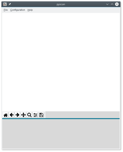
Using ***profiles.nc*** or ***STL*** files cuts through the mesh perpendicular to the X,Y or Z axis can be displayed. This can be used to either check the mesh used for a simulation or the result of the conversion by voxelization process.When **Pyscan** is started without a file name on the command line, a rather blank window is shown:
Pyscan start up window
## 4.1.2. Structure of Menu Bars
## File Menu
* **Open**: Opens the file.
* **Export file**: Exports the data in xlsx formatted files. See below.
* **Export thp data**: Export all **\*thp\*** variables in a plothist file to a xlsx formatted file. This will take some time and might use a lot of memory. It might crash the program. You have been warned.
* **Export particle data**: Export particle related variables in a plothist file to a xlsx formatted file. This will take some time and might use a lot of memory. It might crash the program. You have been warned.
* **Save figure**: Saves the current figure in several formats. This command is different from 'Save the figure' above as it always uses a plot region in A4 size. Because the plot margins are defined in fractions of the plotting area, the settings made under Configure subplots above are also applied here.
* **Dump figures:** For the current profile plot save figures of all time steps to images files. These image files can be used to produce simple movies. This option will take some time.
* **Write netCDF file**: Save the result of the mesh generation to 2 files which can be used as input to GASFLOW-MPI: cadarray.nc and meshgn.txt. cadarray.nc is in NetCDF format. meshgn.txt is readable text. Both filenames can be changed. Additionally a file compatible with VTK (extention .vts) is written to disk with the same name as the result file of the voxelisation. This file can be used in ParaView or VisIt.
* **Write cadarray text file**: Save the result of the mesh generation to 2 files which can be used as input to GASFLOW-MPI: cadarray.txt and meshgn.txt. cadarray.txt contains the same data as before, but as readable text. This file is written as a single line, which can be very long. To write a file with multiple shorter lines, the *linemode* configuration variable can be set to **True**. Additionally a file compatible with VTK (extention .vts) is written to disk with the same name as the result file of the voxelisation. This file can be used in ParaView or VisIt.
* **Quit:** Stop the program.
## **Configuration menu**
### **Plot configuration**
This pop up offers several option to tailor the appearance of the plots. If an option is changed, the changes are not immediately visible. The plot has to be redrawn manually. The pop up has four pages: **Plot**, **Labels**, **Mesh and CAD Import.**
#### **Plot**

If you don't like the *automatic scaling* of the y axis, turn it off and use the 2 entry fields to specify the min. and max. values.
{% hint style="warning" %}
**Warning** this setting will be in effect until it is changed.
{% endhint %}
The *vector scale* parameter is used to determine the length of vectors. The length of the longest vector multiplied by the vector scale is approximately the plot width. In effect: the bigger the vector scale the shorter the vector.
If the vector extends outside the plot area it is clipped. If this is not desired, turn *clip vectors* off.
The *draw grid* option can be used to activate a grid overlay on 2-D plots. The width of the grid lines can specified using the entry field.
#### **Labels**

The parameters in the top line allow to set the *rotation* of the X axis labels, the *size* of the labels (a very small value will produce a default size), and the *color* of the labels for all labeling methods.
The default **grid** labeling algorithm does not always produce satisfying results. It tries to place the labels at the grid locations. It fails if the grid intervals are strongly varying. If this a a problem, either use the **coord** method or specify the grid indices directly using the **custom** method. This **divisor** parameter can be adjusted to change the number of labels generated.
If the **custom** method is selected, you can (and must) specify all indices where a label should be drawn explicitly. You can select the label's colors using the drop down boxes. For the x and y axes there are 2 sets of labels. The second set takes precedence over the first one. This can be used to highlight certain indices by using a different\
color.
The labels have to be specified in a **comma** separated list. Entries ***outside*** the allowed range will be *ignored.* If a list is empty, no label will be drawn with its color.
The indices give the positions, where a label is drawn. Whether an index or a coordinate is used is determined by the "use indices" setting mentioned above.
Because the list can grow longer than the visible space in the entry fields, the buttons at the ends can be used to scroll through the list.
Sometimes even the **custom** method does not work well. In this case the **coord** method might help. It uses the coordinates as the basis for choosing the location of the labels. The *nbins* parameters roughly give the number of intervals on each axis. If the parameter has the value **1,** a default value is chosen. The list of steps can be changed to select different locations. The list must include 1 and 10. Additional values must be between 1 and 10.
#### Mesh

Using the options on this page different colors can be assigned to the object in the displayed mesh.
{% hint style="info" %}
To see the effect of any change, ***redraw***\*\* \*\* the current plot.
{% endhint %}
#### CAD Import

Using the options on this page the voxelization process can be controlled in a more detailed way. Under normal circumstances there should be no need to change the parameters. The directions for the ray casting process can be turned off and on individually as can be the options for the correction of failed rays. At least one ray direction has to be selected to produce a voxelization.
{% hint style="info" %}
Please note: even if a ray fails in one direction, the voxels might be filled by the other two directions. Therefore you might not see any effect of the correction process.
{% endhint %}
The parameters **EPS\_T** and **EPS\_LIMIT** allow to change internal parameters, which can lead to the inclusion or exclusion of triangles of the STL mesh. **EPS\_LIMIT** is added to the bounding box of a triangle. Therefore more triangles might pass the preselection phase. In some cases it might help to set **EPS\_LIMIT** to a small positive value. **EPS\_T** is a parameter for the tolerance in ray direction. It might only help if a triangle is missed at the extreme border of the model. But then it might be better to increase the margin.
## 4.1.3. Mesh Generation
#### Importing STL File to Generate Mesh in Pyscan
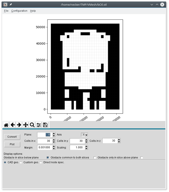
Voxelization using the CAD geometry
If a \_**STL** \_ file is opened using the file menu, below a big blank area a window with two command buttons, **Convert** and **Plot**, will show up. The various parameters to the right of the buttons and below can be used to select the mesh cut for display and to tailor the conversion process.The **Plane** and **Axis** controls select the mesh cut. The 3 **Cells** input fields select the number of cells of the generated mesh in each coordinate direction. The **Margin** input field sets a special parameter for the conversion process. The **Scaling** can be used to convert between the dimension units of the *STL* file and GASFLOW-MPI. The **Display** options can be used to select which items should be displayed.The 3 radio buttons below select 3 different mesh conversion procedures:
* **CAD geo**.: The converted mesh is determined by the outer dimension of model in the *STL* file with the value of the ***Margin*** parameter added. The result is an equidistant mesh.
* **Custom geo**.: The outer dimensions of the generated mesh can be specified directly. If this option is selected after a conversion using **CAD geo**., the values of **CAD geo** are used as initial values. Please note: due to small numerical conversion errors these values will sometimes result in different output. The **Margin** parameter above has to be adjusted to produce a reasonable result.
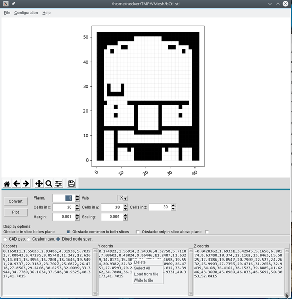
* **Direct node spec**. allows to directly specify the node locations of the generated grid. If the grid generated by **CAD geo** is used as a starting point, some adjustments to the node locations have to be done if the **Margin** parameter is too small. The values in the **X,Y,Z** coords text input areas can be saved as individual text files using the context menu (right mouse button click). In addition copy and paste work too, but only if the text input area is active.
Voxelization using the direct node specification
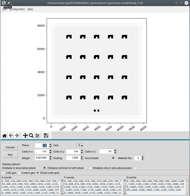
Sometimes it can be advantageous to combine several independent STL files into a single input file for GASFLOW-MPI. This can be achieved by turning on the accumulate mode. See the figure below. The accumulate checkbox has to be turned on *before* the first STL file is converted. The mesh has to match exactly for all STL files to be accumulated. Therefore the nodes have to be specified directly. As long as the accumulate checkbox is checked, the voxelizations of all STL files are remembered and combined when the result file is written to disk. But if one file is voxelized using non-matching coordinates, the list of the previous voxelizations is cleared.The obstacles of the different voxelizations have consecutive material numbers starting from the number in **Material No.**.
Voxelization in accumulate mode
## 4.1.4. Displaying Output
When plothist.nc or profiles.nc files are opened either by specifying the file name on the command line or through the open command the following options are available:
* Plot data to the screen and save the plots in different formats.
* Export the data in *xlsx* format.
The program window is divided into 3 panels:
* the *graphics* panel, where the plots are displayed. This is the big panel at the top.
* the *variable* selection panel at the lower left.
* the *parameter* selection panel at the lower right.
Below the graphics panel, you will notice a short row of seven icons. These are the icons of the standard **matplotlib navigation bar**. Clicking on these icons will activate several functions. From left to right:
* **Home** button: \*\*\*\* reset the view to the state when this pop-up was opened.
* **Back** button: go back one view.
* **Forward** button: forward to next view.
* **Pan/Zoom:** enable pan and zoom. (Try it and if the view is messed up, use the back or home buttons.)
* **Zoom to rectangle:** enable the zoom to rectangle function using the right mouse button.
* **Configure subplots**: Configure the layout of the plot. This button will open a pop-up window, where the margins of the plot can be configured. The pop-up window should be closed, after the adjustments have been done.
* **Save the figure:** Saves the figure into various formats. The size and layout of the figure is as it is currently displayed.
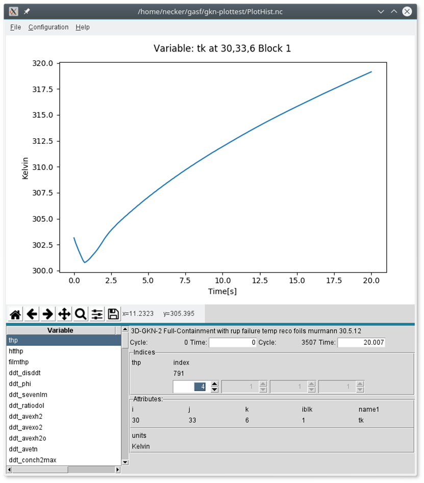
Right to these icons the *current position* in data coordinates is displayed.Depending on the file type, the lower panels have a different content.When **plothist.nc** files are displayed, the panel on the lower left is used to select a variable and the panel on the lower right is used to select the indices of the selected variable.
Displaying Data of plothist.nc
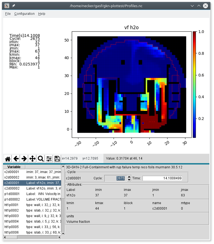
Above the index selection the time span for the display can be selected by entering 2 time values and hitting the Enter/Return key. The closest value present in the file will be selected. All values between these two points in time will be displayed.When **profiles.nc** files are displayed, the panel on the lower left is used to select a variable and the panel on the lower right is used to select the time and the cycle for the plot. The control for the cycle will only assume values present in the file. When a time is input, the program will search the closest value present in the file. If any of the two is changed, the other will show the associated value.If *v2d* or *c2d* plots are displayed, pyscan will print the value at the cursor position right to the above mentioned coordinate display, when the left mouse button is clicked. Please note: for vectors the *start* position of the vector must be clicked on.
Displaying Data of profiles.nc
## 4.1.5. Exporting Data
Using the ***Export data*** command under the **File** menu you can export the underlying data to a file for MS-Excel®, OpenOffice® Calc, LibreOffice® Calc and similiar programs using the xlsx format.
For ***Profiles.nc*** you can export the *currently* displayed data. 2D data are exported using a (x,y,z) format where x,y are the coordinates and z the data.
When viewing time history plots in ***Plothist.nc**,* you can collect several plots into one output file, by pressing **CTRL-c** for each plot to be exported.
{% hint style="warning" %}
*Warning:* Pressing **CTRL-c** multiple times on the same plot will export the data multiple times. Currently there is no indication whether the data have already been selected. If in doubt, simply select the data. In MS-Excel® it is quite easy to delete the unwanted data columns. The first column is the time column. The program will export all values, not only the ones between the two time values mentioned above.
{% endhint %}
To *finally* export the data, you have to select ***Export data*** from the **File** menu.
The following keyboard short cuts are currently implemented:
* Control-q: Quit the program
* Control-Q: Quit the program
* Control-w: Quit the program
* Control-W: Quit the program
* Control-n: Toggle the icon bar below the plot
* Control-s: Save the (current) figure to a file
* Control-S: Save the (current) figure to a file
* Control-c: Collect the exports
* Control-C: Collect the exports
* Control-D: Dump figures
* Control-E: Export thp data
* Control-P: Export particle data
* Control-r: Redraw the current plot using the *current* settings
* Control-R: Redraw the current plot using the *current* settings
{% hint style="info" %}
Remark: a *capital* character in the table above means you have to press a capital character and the control key, i.e. three keys at the time: shift+ctrl+*key*.
{% endhint %}